- ES Español

- EN English

5.24. Numerical Methods (Mandatory)
- Semester: 4th Sem. Credits: 3
- Hour of this course: Theory: 2 hours; Practice: 2 hours;
- Syllabus:
- htmlonly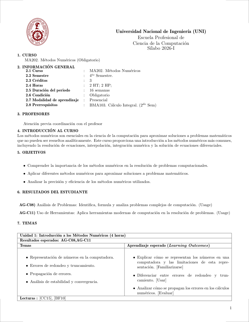
 Español
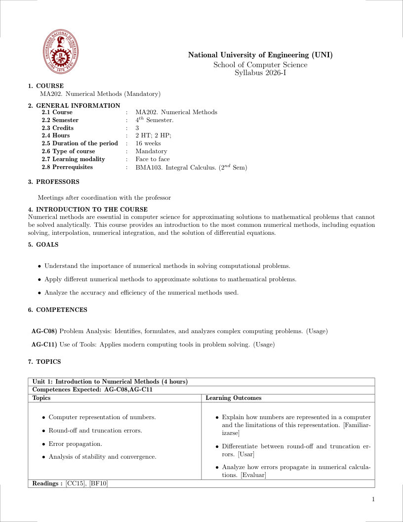 English
 - Prerrequisites:
- BMA103 Integral Calculus (2nd Sem)
5.24.1. Justification ↑ Back to top
Numerical methods are a fundamental tool shared by computer science and engineering disciplines for approximating solutions to mathematical problems that cannot be solved analytically. This course provides an introduction to the most common numerical methods, including error analysis, solution of nonlinear equations, interpolation, numerical integration, and solution of differential equations, in scientific and engineering contexts.
5.24.2. Generales Goals ↑ Back to top
- Understand the importance of numerical methods in solving scientific and engineering problems.
- Apply different numerical methods to approximate solutions to mathematical problems.
- Analyze the accuracy and efficiency of the numerical methods used.
5.24.3. Contribution to Outcomes ↑ Back to top
- AG-C08) Problem Analysis: Identifies, formulates, and analyzes complex computing problems. (Usage)
- AG-C11) Use of Tools: Applies modern computing tools in problem solving. (Usage)
- AG-C09) Design and Development of Solutions: Designs, implements, and evaluates solutions for complex computing problems. (Usage)
5.24.4. Content ↑ Back to top
5.24.4.1. Error Analysis and Floating-Point Arithmetic (6 hours) [Skills AG-C08,AG-C11] ↑ Back to top
Bibliography: (Chapra and Canale, 2015; Burden and Faires, 2010)
Topics
- IEEE 754 floating-point representation: machine epsilon, overflow, underflow, and rounding modes
- Rounding errors, catastrophic cancellation, and loss of significance
- Forward and backward error analysis; condition number of a problem
- Numerical stability: stable vs. unstable algorithms; Wilkinson's backward error analysis
- Error propagation in arithmetic operations and function evaluation
Learning Outcomes
- Explain the IEEE 754 floating-point standard and identify the sources of rounding and cancellation errors [Familiarity]
- Estimate the condition number of a problem and predict the accuracy of a numerical result [Usage]
- Analyze an algorithm for numerical stability using forward and backward error bounds [Assessment]
5.24.4.2. Root-Finding for Nonlinear Equations (10 hours) [Skills AG-C08,AG-C11] ↑ Back to top
Bibliography: (Chapra and Canale, 2015; Burden and Faires, 2010)
Topics
- Bisection method: interval bracketing, stopping criteria, and error bound
- Newton-Raphson method: derivation, quadratic convergence, and failure cases
- Secant method as an alternative to Newton's method without an explicit derivative
- Order of convergence and efficiency comparison among iterative methods
- Extension of Newton's method to systems of nonlinear equations via the Jacobian matrix, the basis of solvers used in machine learning
Learning Outcomes
- Compare the convergence guarantees of the bisection, Newton-Raphson, and secant methods [Familiarity]
- Implement the Newton-Raphson method to approximate roots of a nonlinear function [Usage]
- Analyze the order of convergence of an iterative method and justify its choice based on computational cost [Assessment]
5.24.4.3. Approximation Theory and Interpolation (10 hours) [Skills AG-C08,AG-C11] ↑ Back to top
Bibliography: (Chapra and Canale, 2015; Burden and Faires, 2010)
Topics
- Polynomial interpolation: Lagrange, Newton divided differences, and Runge's phenomenon
- Spline interpolation: cubic splines, B-splines, and piecewise polynomial methods
- Best approximation in normed spaces: Chebyshev (minimax) and least squares
- Chebyshev polynomials: properties, orthogonality, and spectral convergence
- Trigonometric approximation and the fast Fourier transform (FFT)
Learning Outcomes
- Explain Runge's phenomenon and justify the choice of Chebyshev nodes to mitigate it [Familiarity]
- Construct cubic spline and Chebyshev interpolants for given data and estimate the interpolation error [Usage]
- Apply the FFT to efficiently compute trigonometric approximations of a sampled function [Assessment]
5.24.4.4. Numerical Integration and Quadrature (10 hours) [Skills AG-C08,AG-C11] ↑ Back to top
Bibliography: (Chapra and Canale, 2015; Burden and Faires, 2010)
Topics
- Newton-Cotes rules: trapezoidal, Simpson's, and composite rules; error analysis
- Adaptive quadrature and automatic error control
- Gaussian quadrature: optimal nodes and weights, orthogonal polynomial connection
- Numerical treatment of improper and singular integrals
- Monte Carlo integration and quasi-Monte Carlo methods for high-dimensional integrals
Learning Outcomes
- Derive the error formula for composite Simpson's rule and identify its order of accuracy [Familiarity]
- Select and apply an appropriate quadrature rule (Gaussian, adaptive) based on integrand regularity [Usage]
- Apply Monte Carlo integration to estimate high-dimensional integrals and quantify the statistical error [Assessment]
5.24.4.5. Numerical Methods for Differential Equations (12 hours) [Skills AG-C08,AG-C11] ↑ Back to top
Bibliography: (Chapra and Canale, 2015; Burden and Faires, 2010)
Topics
- Runge-Kutta methods: Euler, RK4, and embedded methods for error control
- Linear multistep methods: Adams-Bashforth, Adams-Moulton, and BDF methods
- Stability analysis: zero-stability, absolute stability regions, and stiff ODEs
- Finite difference methods for parabolic and elliptic PDEs: stability and convergence
Learning Outcomes
- Compare explicit and implicit ODE solvers and explain their relative stability for stiff problems [Familiarity]
- Implement a Runge-Kutta method with adaptive step control and apply it to a system of ODEs [Usage]
- Analyze the stability and convergence of a finite difference scheme for a parabolic PDE [Assessment]
5.24.4.6. Numerical Linear Algebra (12 hours) [Skills AG-C08,AG-C11] ↑ Back to top
Bibliography: (Burden and Faires, 2010; Trefethen and III, 1997)
Topics
- Gaussian elimination with partial pivoting, LU factorization, and complexity analysis
- QR factorization via Householder and Gram-Schmidt; least squares problems
- Eigenvalue algorithms: power iteration, QR algorithm, and the Lanczos method
- Singular value decomposition: computation, truncation, and applications (PCA, pseudoinverse)
- Iterative methods for large sparse systems: CG, GMRES, and preconditioning
Learning Outcomes
- Compare direct and iterative solvers and select the appropriate method for a given matrix structure [Familiarity]
- Apply QR factorization and SVD to solve least squares problems and compute low-rank approximations [Usage]
- Analyze the numerical stability and computational cost of eigenvalue algorithms [Assessment]
5.24.4.7. Finite Element Method (8 hours) [Skills AG-C08,AG-C09] ↑ Back to top
Bibliography: (Reddy, 2019; Burden and Faires, 2010)
Topics
- Weak (variational) formulation of boundary value problems and Sobolev spaces
- Galerkin method: finite-dimensional approximation spaces and the stiffness matrix
- Triangular and quadrilateral finite element spaces: Lagrange elements and conformity
- A priori error estimates: Céa's lemma and interpolation error bounds
- A posteriori error estimates and adaptive mesh refinement
Learning Outcomes
- Derive the weak formulation of an elliptic BVP and show its equivalence to the strong form [Familiarity]
- Assemble the global stiffness matrix and load vector for a linear finite element discretization [Usage]
- Estimate the \(H^1\) error of a finite element solution using Céa's lemma and interpolation theory [Assessment]
5.24.4.8. Optimization Algorithms (4 hours) [Skills AG-C09,AG-C11] ↑ Back to top
Bibliography: (Nocedal and Wright, 2006)
Topics
- Gradient descent and line search methods: Armijo-Wolfe conditions and convergence rates
- Newton's method and quasi-Newton methods (BFGS, L-BFGS)
- Constrained optimization: KKT conditions, penalty methods, and sequential quadratic programming
- Convex optimization algorithms: interior-point methods and ADMM
- Stochastic gradient descent (SGD), variance reduction, and Adam optimizer
Learning Outcomes
- Explain the convergence guarantees of gradient descent for smooth convex functions [Familiarity]
- Apply Newton and quasi-Newton methods to unconstrained optimization problems [Usage]
- Formulate a constrained optimization problem as a KKT system and apply an interior-point method [Assessment]
5.24.4.9. Parallel and High-Performance Computing (4 hours) [Skills AG-C11] ↑ Back to top
Bibliography: (Pacheco and Malensek, 2022)
Topics
- Parallel architectures: shared memory (OpenMP), distributed memory (MPI), and GPU (CUDA)
- Performance models: Amdahl's law, roofline model, and communication complexity
- Parallel algorithms for dense and sparse linear algebra (ScaLAPACK, PETSc)
- Domain decomposition and parallel PDE solvers
- Automatic differentiation (forward and reverse mode) and its role in scientific ML
Learning Outcomes
- Explain Amdahl's law and identify the bottlenecks limiting parallel speedup in a given algorithm [Familiarity]
- Implement a parallel linear algebra routine using MPI or OpenMP and measure parallel efficiency [Usage]
- Apply automatic differentiation to compute gradients of complex scientific functions for optimization [Assessment]
5.24.4.10. Graph Theory (4 hours) [Skills AG-C08] ↑ Back to top
Bibliography: (West, 2001)
Topics
- Graphs: definitions, isomorphism, degree sequences, trees, and spanning trees
- Connectivity, Menger's theorem, and network flows (max-flow min-cut)
- Matchings (Hall's theorem), graph colorings, and the chromatic polynomial
- Planar graphs, Euler's formula, Kuratowski's theorem, and the four-color theorem
- Adjacency and Laplacian matrices, eigenvalues, and expander graphs
Learning Outcomes
- Identify structural properties of graphs (connectivity, planarity, bipartiteness) and apply Euler's formula [Familiarity]
- Apply Hall's marriage theorem and network flow algorithms to matching and routing problems [Usage]
- Analyze a graph's spectrum to bound its chromatic number and connectivity properties [Assessment]
5.24.4.11. Time Series Analysis (2 hours) [Skills AG-C08,AG-C11] ↑ Back to top
Bibliography: (Shumway and Stoffer, 2017)
Topics
- Stationarity, autocovariance function, and the autocorrelation function (ACF)
- ARMA models: identification, estimation (Yule-Walker, MLE), and diagnostics
- Spectral density, the periodogram, and Wiener-Khinchin theorem
- State-space models and the Kalman filter
- ARIMA models, seasonal adjustment, and multi-step forecasting
Learning Outcomes
- Identify stationarity and determine the order of an ARMA model from ACF and PACF plots [Familiarity]
- Fit ARIMA models to time series data, validate residuals, and produce forecasts [Usage]
- Apply the Kalman filter to estimate hidden states in a linear Gaussian state-space model [Assessment]
5.24.5. Bibliography ↑ Back to top
Chapra, S. C. and Canale, R. P. (2015). Numerical Methods for Engineers. McGraw-Hill Education.
Burden, R. L. and Faires, J. D. (2010). Numerical Analysis. Cengage Learning.
Trefethen, L. N. and III, D. B. (1997). Numerical Linear Algebra. SIAM.
Reddy, J. N. (2019). An Introduction to the Finite Element Method. McGraw-Hill Education, 4th edition.
Nocedal, J. and Wright, S. J. (2006). Numerical Optimization. Springer, 2nd edition.
Pacheco, P. S. and Malensek, M. (2022). An Introduction to Parallel Programming. Morgan Kaufmann, 2nd edition.
West, D. B. (2001). Introduction to Graph Theory. Prentice Hall, 2nd edition.
Shumway, R. H. and Stoffer, D. S. (2017). Time Series Analysis and Its Applications: With R Examples. Springer, 4th edition.